Getting started with ngspice can be quite tricky. It’s a very powerful piece of software and although the user manual is quite comprehensive, its complexity can easily scare off beginners.
Here’s a simple step-by-step tutorial on how to simulate a very simple electronic circuit. It should enable you to run your own simulations of circuits you designed.

Creating the circuit

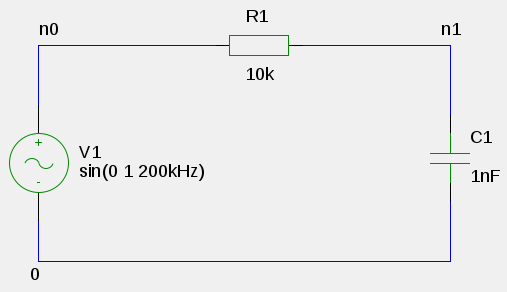
The sample circuit is a lowpass RC filter. It’s simple, contains a reasonable amount of components and yet we can do different types of analysis. I assume, you already know how to use gschem. If not, have a look at the gEDA wiki for a list of tutorials.

Start up gschem and draw the following circuit:

Simple lowpass RC filter

Of course, you can name your buses differently. I chose n0 and n1 here. The bus named 0 is mandatory as it specifies the reference (ground) net.

V1 is an independent AC voltage source. It’s parameters are wave form (sin), voltage offset in Volts (0[V]), amplitude in Volts (1[V]) and frequency (200kHz).

Save the schematic as rcSIN.sch.

Generating the netlist

SPICE doesn’t use gschem schematics as input but so-called netlists. To generate a netlist file from a schematic, gnetlist can be used:

$ gnetlist -g spice -o rcSIN.net rcSIN.sch 
Command line passed = gnetlist -g spice -o rcSIN.net rcSIN.sch 
Loading schematic [rcSIN.sch]

The resulting rcSIN.net should look like this:

* Spice netlister for gnetlist
R1 n1 n0 10k
C1 n1 0 1nF
V1 n0 0 sin(0 1 200kHz)
.END

The file is quite self-explanatory: Each line contains a single component, the first column of each line the component’s reference designator, the subsequent columns the netnames for each pin and finally the value attribute.

Running a transient simulation

SPICE can run different types of analysis, e.g.

• A transient analysis shows how the circuit behaves over time
• An AC analysis shows the behaviour of the circuit with varying frequency
• A parametrized analysis can be either a transient or an AC analysis. It varies one or more values of a given circuit, e.g. the resistance of a Resistor.

Let’s run a transient analysis first. Start up ngspice

$ ngspice 
******
** ngspice-23 : Circuit level simulation program
** The U. C. Berkeley CAD Group
** Copyright 1985-1994, Regents of the University of California.
** Please get your ngspice manual from http://ngspice.sourceforge.net/docs.html
** Please file your bug-reports at http://ngspice.sourceforge.net/bugrep.html
** Creation Date: Sat Jan 14 14:20:54 UTC 2012
******
ngspice 230 -> 

and load the netlist file

ngspice 230 -> source rcSIN.net

Circuit: * spice netlister for gnetlist

ngspice 231 -> 

Our voltage source runs at a frequency of \(200kHz\), which means our oscillating period is \(200kHz^{-1} = 5{\mu}s\). Let’s say, we want to see how the input voltages behaves during the first 5 oscillations (i.e. \(5 \cdot 5{\mu}s = 25{\mu}s\)) and we want to have a data point every \(0.05{\mu}s\):

ngspice 231 -> tran 0.05us 25us
Doing analysis at TEMP = 27.000000 and TNOM = 27.000000

Warning: v1: no DC value, transient time 0 value used

Initial Transient Solution
--------------------------

Node                                   Voltage
----                                   -------
n1                                           0
n0                                           0
v1#branch                                    0

%100.00

No. of Data Rows : 508
ngspice 232 -> 

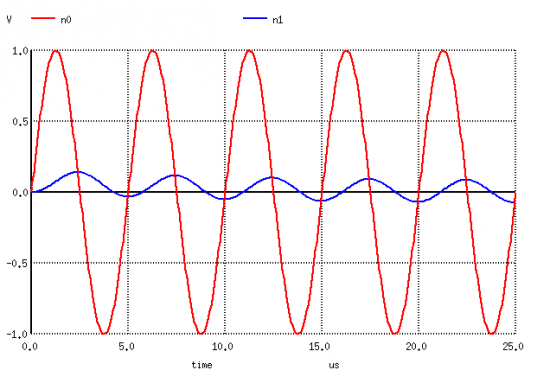
We can now plot the results:

ngspice 232 -> plot n0 n1

Output graph of the transient analysis

Running an AC simulation

You can easily see that the signal at the resistor R1 is significantly smaller as the input voltage. Of course, you can adjust the values for R1 and C1 to archive even lower signal levels, but the signal level is also determined by the input frequency. So let’s run and AC analysis to see how the RC filter behaves when we alter the input frequency.

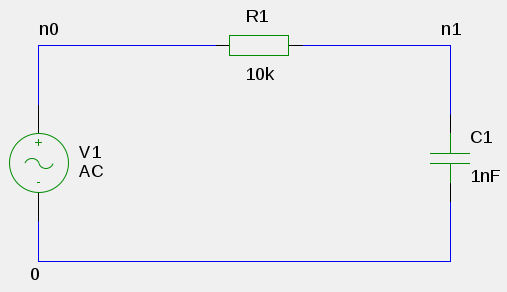
Open up gschem again and change the input voltage to AC:

Changed input voltage (AC)

Save the schematic as rcAC.sch and generate a netlist file (rcAC.net)

$ gnetlist -g spice -o rcAC.net rcAC.sch 
Command line passed = gnetlist -g spice -o rcAC.net rcAC.sch 
Loading schematic [rcAC.sch]

We are now ready to run an AC analysis. For a detailed explanation of the ac command syntax, have a look at “SPICE – A Brief Tutorial”. Don’t forget to load the rcAC.net netlist file before you run the analysis!

ngspice 236 -> source rcAC.net

Circuit: * spice netlister for gnetlist

ngspice 237 -> ac lin 1000 0.1 250kHz
Doing analysis at TEMP = 27.000000 and TNOM = 27.000000

Warning: v1: has no value, DC 0 assumed


No. of Data Rows : 1000
ngspice 238 -> plot n0 n1
ngspice 239 -> 

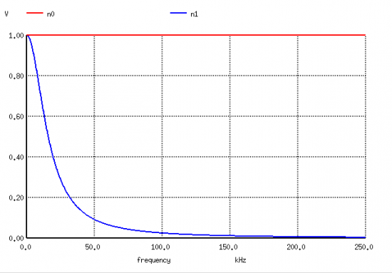
This command performs a linear frequency analysis (lin) from (almost) 0Hz to 250kHz and generates 1000 data points. To view the results, plot the input voltage and the voltage over R1 versus the frequency:

Frequency analysis

Have a look at http://ashwith.wordpress.com/2010/09/30/ngspice-interactive-mode/ for more ngspice examples.

Schematic and netlist files:
rcSIN.sch rcSIN.net rcAC.sch rcAC.net